c03_ridge_joyplot 数据分布 (Distribution)
Nature Cell Lancet
High-Density Ridge / Joyplot
高密度山峦脊线图 (Ridge / Joyplot),展示连续变量在不同类别或时间周期上的分布形态漂移。
🔬 矢量预览 (Vector Preview)
600 DPI Ready
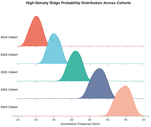
格式支持: SVG, PDF, PNG (600 DPI), TIFF
📊 统计学特性 (Statistical Features)
- ✓ 高斯核密度估计 (Gaussian KDE)
- ✓ 重叠阶梯面积渲染
- ✓ 基线零线对齐
- ✓ 透明度色彩叠加
🛡️ QC 质检要点 (QC Highlights)
- ✓ 重叠度适中 (0.4-0.6) 无完全遮挡
- ✓ Y 轴类别标签水平对齐
- ✓ X 轴单位标注完整
- ✓ 打印灰度可辨识
🎨 顶刊色彩提取器 (Palette Extractor)Nature
Crisp sans-serif typography, clean borderless spines, high-contrast palette with soft muted secondary accents.
🛡️ 无障碍评分:AAA (Deuteranopia & Protanopia Compliant)
📋 Data Contract 数据契约规范 Strict Schema
输入数据必须完全符合下列列名与数据类型规范,方可通过自动化数据前检 (Pre-flight Validation)。
| 字段名称 (Column) | 数据类型 (Type) | 约束性 | 语义说明与值域约束 |
|---|---|---|---|
| cohort | categorical | 必需 (Required) | Ordered grouping category or temporal epoch |
| value | continuous | 必需 (Required) | Continuous response metric to evaluate probability density |
| weight | continuous | 可选 (Optional) | Optional sample weight for weighted KDE |
组内最小样本量: n ≥ 5
最大允许缺失率: 5%
🐍 独立可复现 Python 绘图源码 Stand-alone Script
完全可复现的 Python 脚本,支持 CLI 参数 `--data`, `--style`, `--output-dir` 与模块化 `render()` 调用。
#!/usr/bin/env python3
"""FigureCraft Chart Engine: High-Density Ridge / Joyplot (c03_ridge_joyplot)."""

import os
import sys
import argparse
from pathlib import Path
from typing import List, Dict, Optional
import numpy as np
import pandas as pd
import matplotlib.pyplot as plt
from scipy import stats

try:
    from engines.styles import apply_style, get_palette
except ImportError:
    sys.path.insert(0, str(Path(__file__).resolve().parents[2]))
    from engines.styles import apply_style, get_palette

CHART_ID = "c03_ridge_joyplot"


def render(
    data_path: Optional[str] = None,
    style: str = "nature",
    output_dir: str = "output",
    formats: Optional[List[str]] = None,
    dpi: int = 600,
) -> Dict[str, str]:
    if formats is None:
        formats = ["svg", "pdf", "png", "tiff"]
    if data_path is None:
        data_path = str(Path(__file__).resolve().parents[1] / "data" / f"{CHART_ID}.csv")

    apply_style(style)
    palette = get_palette(style)
    df = pd.read_csv(data_path)
    df = df.dropna(subset=["cohort", "value"])

    cohorts = list(df["cohort"].unique())
    k = len(cohorts)

    # Compute global x range
    x_min = df["value"].min() - (df["value"].max() - df["value"].min()) * 0.1
    x_max = df["value"].max() + (df["value"].max() - df["value"].min()) * 0.1
    x_eval = np.linspace(x_min, x_max, 250)

    fig, axes = plt.subplots(
        nrows=k,
        ncols=1,
        figsize=(6.5, 4.8),
        sharex=True,
        gridspec_kw={"hspace": -0.45},
    )

    if k == 1:
        axes = [axes]

    for i, (ax, cohort) in enumerate(zip(axes, cohorts)):
        cohort_vals = df[df["cohort"] == cohort]["value"].values
        color = palette[i % len(palette)]

        if len(cohort_vals) >= 2:
            kde = stats.gaussian_kde(cohort_vals, bw_method="silverman")
            y_density = kde(x_eval)
        else:
            y_density = np.zeros_like(x_eval)

        # Baseline white mask to prevent bleed-through
        ax.fill_between(x_eval, 0, y_density, color="#FFFFFF", alpha=1.0, zorder=2)
        # Colored KDE fill
        ax.fill_between(x_eval, 0, y_density, color=color, alpha=0.75, zorder=3)
        # Top boundary line
        ax.plot(x_eval, y_density, color=color, linewidth=1.2, zorder=4)

        # Baseline reference line
        ax.axhline(0, color="#D1D5DB", linewidth=0.6, zorder=1)

        # Left label for cohort
        ax.text(
            x_min,
            np.max(y_density) * 0.25 if np.max(y_density) > 0 else 0.05,
            cohort.replace("_", " "),
            fontsize=7.5,
            fontweight="bold",
            color="#1F2937",
            ha="right",
            va="bottom",
        )

        # Clean background & hide unnecessary spines
        ax.patch.set_alpha(0.0)
        ax.set_ylim(bottom=0)
        ax.set_yticks([])
        for spine in ["top", "right", "left", "bottom"]:
            ax.spines[spine].set_visible(False)

    # Enable bottom spine and x-ticks on bottom axis
    axes[-1].spines["bottom"].set_visible(True)
    axes[-1].spines["bottom"].set_color("#111827")
    axes[-1].spines["bottom"].set_linewidth(0.5)
    axes[-1].tick_params(bottom=True, labelbottom=True, labelsize=7.5)
    axes[-1].set_xlabel("Quantitative Response Metric", fontsize=8.0)

    fig.suptitle("High-Density Ridge Probability Distribution Across Cohorts", fontsize=9.5, fontweight="bold", y=0.98)

    os.makedirs(output_dir, exist_ok=True)
    generated_files = {}
    for fmt in formats:
        out_path = os.path.join(output_dir, f"{CHART_ID}_{style}.{fmt}")
        fig.savefig(out_path, format=fmt, dpi=dpi, bbox_inches="tight")
        generated_files[fmt] = str(Path(out_path).resolve())

    plt.close(fig)
    return generated_files


if __name__ == "__main__":
    parser = argparse.ArgumentParser(description="Render High-Density Ridge / Joyplot")
    parser.add_argument("--data", type=str, default=None, help="Path to input CSV dataset")
    parser.add_argument("--style", type=str, default="nature", choices=["nature", "cell", "lancet", "ieee", "economist"], help="Journal style pack")
    parser.add_argument("--output-dir", type=str, default="output", help="Output directory")
    parser.add_argument("--formats", type=str, default="svg,pdf,png,tiff", help="Comma-separated export formats")
    parser.add_argument("--dpi", type=int, default=600, help="Raster DPI")
    args = parser.parse_args()

    fmt_list = [f.strip() for f in args.formats.split(",") if f.strip()]
    results = render(args.data, style=args.style, output_dir=args.output_dir, formats=fmt_list, dpi=args.dpi)
    for fmt, path in results.items():
        print(f"Generated {fmt.upper()}: {path}")